I’m going to start with a little history of the support vector machines (SVM) and why they are so common in neuroimaging classification. It was first introduced by Vladimir Vapnik, implemented Bernhard Boser, and Isabelle Guyon suggested using kernels to Vladmir and thus the many flavors of SVM was born. Why SVM have risen to prominence in neuroimaging isn’t so clear but there are some reasons suggesting why. SVM are relatively easy to interpret compared to other machine learning algorithms. A linear decision boundary (usually) makes sense and is intuitive. The algorithm has the design to let misclassifications exist in a model and helps make the decision boundary better. This makes it robust and not run astray when there are many observations that are misclassified, which is often the case. Probably the biggest reason is that scientists saw SVM were working and from there it caught fire within the neuroimaging community.
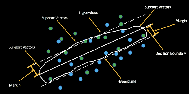
Now to the actual algorithm. Actually, lets start with support vector classifiers (SVC). This is a SVM without a kernel. Let’s build this algorithm up. SVC project features into what we’ll call a hyperplane and this is a p-dimensional space (feature space). In two dimensions, the hyperplane is flat one-dimensional subspace and builds up from there. There are several key terms to know:
*Decision boundary: Boundary deciding which class each observation belongs to.
*Support Vectors: Observations that influence the location of the decision boundary.
*Margin: the smallest distance from the observations to the hyperplane.
*Slack Variables: Allows individual observations to be on the wrong side of the margin or hyperplane.
**C controls the margins. The smaller it is, the smaller the margins are thus less violations to the margins (small amount of support vectors).
**Gamma controls how much influence far away support vectors have. The larger the value, the less influence far away support vectors have. If it’s large, then model will have more bias and low variance.
A kernel is a math trick that transforms the feature space allowing for a linear decision boundary to be created and then transformed back into the original feature space to give a kind of non-linear decision boundary like a circle or polynomial. A Kernel can be defined as a function quantifying the similarity between two observation. I’m not going to talk more about them because that could be a whole other blog post.
I’m going to briefly talk about tuning the slack variables. In some cases it actually may be best to not tune your model e.g. non-sparse decoders. In the case of my tutorial, I use a sort of sparse decoder by applying L1 regularization before the model, which IMO practically makes it a sparse decoder. The best way to tune these parameters is through cross-validation. This will select the parameters based off which pair of slack variables had the lowest MSE. This is easy to implement and empirically justifies your parameters for your model.
Putting it all together, you want to think about what kind of questions you are trying to answer with your model. Are you only trying to get a high classification accuracy or are you also trying to have some interpretability in your model? This is essentially a bias-variance trade off question for your model which you should be keeping in mind while designing your model.