ANOVAs are handy, however, are limited by the number of variables the model can handle. I.e. you can only test two variables across groups. Multiple Analysis of Variance (MANOVA) models can handle this problem.
MANOVA
MANOVA is an extension of the ANOVA so it’ll be helpful for you if you’ve familiarized yourself with it. It will also be helpful if you’ve familiarized yourself with matrix maths. Because we’re dealing with a more complex model it’s helpful to use matrices to solve it.
Let’s imagine for each observation e.g. each participant, is modeled as vectors where $$y_{ij} = \mu + \epsilon_{ij}$$ where $$i = 1, 2, … , k;$$ is the variable, $$j = 1, 2, …, n.$$ is the $\mu_i$ is the group mean and $\epsilon_{ij}$ is the error for that variable and observation. As in the ANOVA, the null hypothesis in a MANOVA is still $H0: \mu_1 = \mu_2 = \mu_3$ and the alternate hypothesis is $H0: \mu_1 \neq \mu_2 \neq \mu_3$.
Wilks’ Test Statistic
$$\Lambda = \frac{|E|}{|E + H|}$$
We reject $H_0$ if $\Lambda \underline{<} \Lambda_{\alpha, p, \upsilon H, \upsilon E}$ where p is the number of variables, $\upsilon H$ is the degrees of freedom for the hypothesis, and $\upsilon E$ is the degrees of freedom for error. This is analogous to the F test in the ANOVA. R nicely calculates the analgous F-statistic for us so I’m not going to go into how that’s calculated.
To calculate the between sample variance matrix: ($H$) is $$H = \sum_{i=1}^k\frac{1}{n}y_{i}y\prime_i - \frac{1}{kn}yy\prime$$. To calculate within sample variance matrix ($E$) is $$E = \sum_{ij}y_{ij}y\prime_{ij} - \sum_i \frac{1}{n}y_iy\prime_i$$.
Now we can calculate $\Lambda$ and get the F stastistic.
In R:
#install.packages("car")
library(car)
## Loading required package: carData
data(iris)
man.model = manova(cbind(Sepal.Length, Sepal.Width, Petal.Length) ~ Species, data = iris)
res.man=summary(manova(cbind(Sepal.Length, Sepal.Width, Petal.Length) ~ Species, data = iris), test = "Wilks")
res.man
##            Df    Wilks approx F num Df den Df    Pr(>F)
## Species     2 0.031546    223.8      6    290 < 2.2e-16 ***
## Residuals 147
## ---
## Signif. codes:  0 '***' 0.001 '**' 0.01 '*' 0.05 '.' 0.1 ' ' 1
Great we rejected the null for the overall model, what about each variable? To this we have to do post-hoc testing to compare each variable within each group. This is the same as what we did in the ANOVA. I’ll use Tukey’s HSD for the post-hocs.
In R:
#devtools::install_github("easystats/report")
#install.packages("ggplot2)
#install.packages("dplyr")
library(report)
library(ggplot2)
library(dplyr)
##
## Attaching package: 'dplyr'
## The following object is masked from 'package:car':
##
##     recode
## The following object is masked from 'package:kableExtra':
##
##     group_rows
## The following objects are masked from 'package:stats':
##
##     filter, lag
## The following objects are masked from 'package:base':
##
##     intersect, setdiff, setequal, union
Contrasts
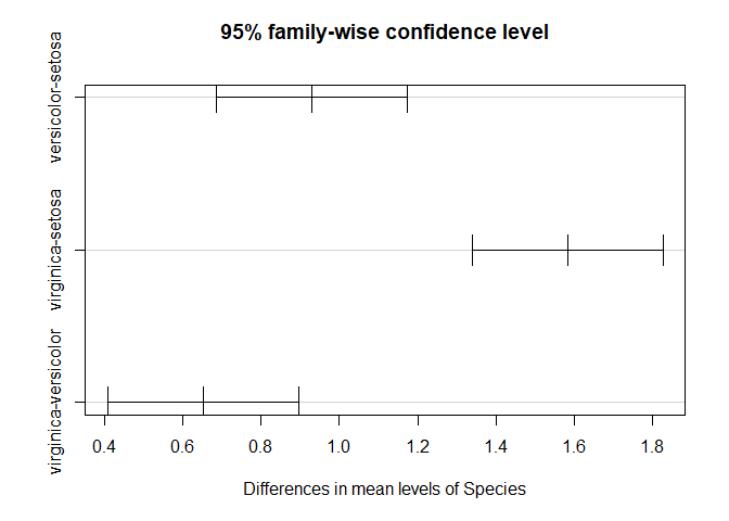
1. Sepal Length Here, we’ll test differences in sepal length between the three species.
fit.s.length <- aov(Sepal.Length ~ Species, data=iris)
summary(fit.s.length)
##              Df Sum Sq Mean Sq F value Pr(>F)
## Species       2  63.21  31.606   119.3 <2e-16 ***
## Residuals   147  38.96   0.265
## ---
## Signif. codes:  0 '***' 0.001 '**' 0.01 '*' 0.05 '.' 0.1 ' ' 1
fit.s.length %>%
  report() %>%
  to_table()
##   Parameter Sum_Squares DoF Mean_Square        F            p
## 1   Species    63.21213   2  31.6060667 119.2645 1.669669e-31
## 2 Residuals    38.95620 147   0.2650082       NA           NA
##   Omega_Sq_partial
## 1        0.6119308
## 2               NA
TukeyHSD(fit.s.length)
##   Tukey multiple comparisons of means
##     95% family-wise confidence level
##
## Fit: aov(formula = Sepal.Length ~ Species, data = iris)
##
## $Species
##                       diff       lwr       upr p adj
## versicolor-setosa    0.930 0.6862273 1.1737727     0
## virginica-setosa     1.582 1.3382273 1.8257727     0
## virginica-versicolor 0.652 0.4082273 0.8957727     0
plot(TukeyHSD(fit.s.length))
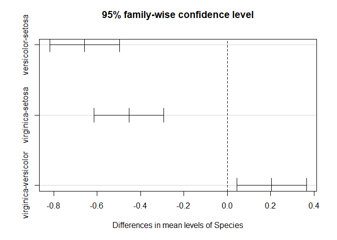
2. Sepal Width Here, we’ll test differences in sepal width between the three species.
fit.s.width <- aov(Sepal.Width ~ Species, data=iris)
fit.s.width %>%
  report() %>%
  to_table()
##   Parameter Sum_Squares DoF Mean_Square        F            p
## 1   Species    11.34493   2   5.6724667 49.16004 4.492017e-17
## 2 Residuals    16.96200 147   0.1153878       NA           NA
##   Omega_Sq_partial
## 1        0.3910362
## 2               NA
TukeyHSD(fit.s.width)
##   Tukey multiple comparisons of means
##     95% family-wise confidence level
##
## Fit: aov(formula = Sepal.Width ~ Species, data = iris)
##
## $Species
##                        diff         lwr        upr     p adj
## versicolor-setosa    -0.658 -0.81885528 -0.4971447 0.0000000
## virginica-setosa     -0.454 -0.61485528 -0.2931447 0.0000000
## virginica-versicolor  0.204  0.04314472  0.3648553 0.0087802
plot(TukeyHSD(fit.s.width))
3. Petal.Length Here, we’ll test differences in petal length between the three species.
fit.p.length <- aov(Petal.Length ~ Species, data=iris)
summary(fit.p.length)
##              Df Sum Sq Mean Sq F value Pr(>F)
## Species       2  437.1  218.55    1180 <2e-16 ***
## Residuals   147   27.2    0.19
## ---
## Signif. codes:  0 '***' 0.001 '**' 0.01 '*' 0.05 '.' 0.1 ' ' 1
fit.p.length %>%
  report() %>%
  to_table()
##   Parameter Sum_Squares DoF Mean_Square        F            p
## 1   Species    437.1028   2 218.5514000 1180.161 2.856777e-91
## 2 Residuals     27.2226 147   0.1851878       NA           NA
##   Omega_Sq_partial
## 1        0.9401991
## 2               NA
TukeyHSD(fit.p.length)
##   Tukey multiple comparisons of means
##     95% family-wise confidence level
##
## Fit: aov(formula = Petal.Length ~ Species, data = iris)
##
## $Species
##                       diff     lwr     upr p adj
## versicolor-setosa    2.798 2.59422 3.00178     0
## virginica-setosa     4.090 3.88622 4.29378     0
## virginica-versicolor 1.292 1.08822 1.49578     0
plot(TukeyHSD(fit.p.length))
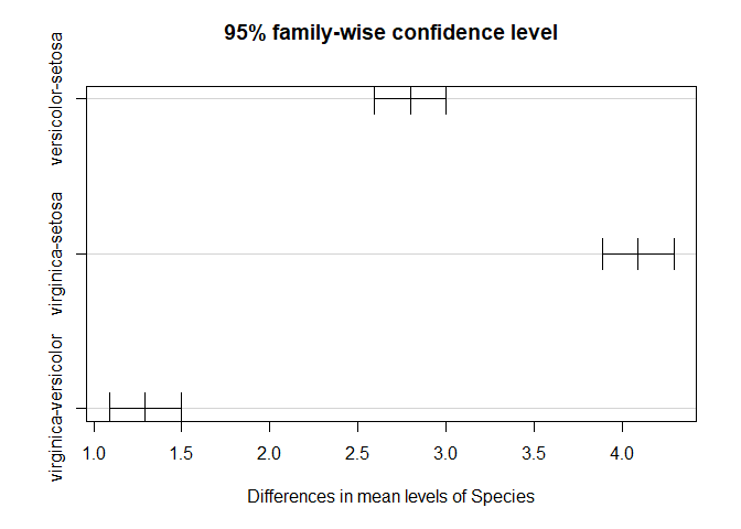
As expected all of the variables across all groups are siginificant.
A slight aside in confusing terminology that came up while I was doing this. Contrasts and post-hocs are different. Contrasts are when you have a planned test even if, in this case a MANOVA, was not significant. Although, typically you accect the results of the MANOVA regardless if your contrasts are significant. Post-hocs are only done when you don’t have an apriori hypothesis test between two variables and if the MANOVA was significant.
In the next post, I’ll discuss ANCOVAs.
References
https://www.r-bloggers.com/multiple-analysis-of-variance-manova/