The ridge regression (L2 penalization) is similar to the lasso (L1 regularization), and the ordinary least squares (OLS) regression. In this post I will discuss some differences between L2 and L1 regressions, and how to do this R. This post will be pretty similar to my lasso post.
The ridge is just another regression and can be quite useful in machine learning. It penalizes features (variables) that are redundant or are not associated with the Y variable you are trying to predict. It’s really nothing wild. Let me put it this way, if you can understand $Y = mx + b$, you can understand any regression (Nick Lazich, 2017). This holds true for the ridge.
Let’s start with the (OLS) equation or better known as a linear regression that we’re all familiar with. If you aren’t, take a peak here. Straight forward enough. $$Y = \beta_0 + \beta_1X_1 + \beta_2X_2 + … \beta_n+X_n + \mu$$
Which may also look like -
$$L_{OLS} = ||y - X\hat{\beta}||^2$$
And to get the beta estimate (beta hat), all it is the covariance between x and y divided by the variance of x. This beta estimate is then plugged back into the equation above and your on your way to predicting that sweet sweet Y-value.
$$\hat{\beta} = \frac{\sum_{i=1}^n(y_i - \overline{y})(x_i - \overline{x})}{\sum_{i=1}^n(x_i - \overline{x})^2}$$
And further -
$$\hat{\beta}_{OLS} = (X’X)^{-1}(X’Y)$$
This annotation is helpful for cases when there is more than one $\beta$ which is pretty much always the case. Moral of the story is matrix maths.
Let’s make this beta estimate a wee bit more complicated -
$$\hat{\beta}_{ridge} = argmin_{\beta \epsilon R} \left.||y - X \hat{\beta} \right||^{2} + \left. \lambda|| \hat{\beta} \right||^{2}$$
Okay, the equation might look a little intimidating - let’s simplify it a little more -
$$\hat{\beta}_{ridge} = (X’X + \lambda I)^{-1}(X’Y)$$
I denotes the identity matrix. $\lambda$ is the penalization factor that we can set beforehand. The larger it is, the more penalization on your features and the smaller it is, the less penalization on your features. If $\lambda = 0$, it actually becomes an OLS regression.
You might be wondering how come the ridge doesn’t do feature selection like the lasso by pushing features to 0. Due to the matrix maths involved, the $\lambda$ ends up in denominator and we all know we can’t divide by 0. Thus the features are never pushed to 0 but can come very close, unlike the lasso.
Okay let’s try this in R.
#install.package(glmnet) - install this if you don't have it already
#install.package(caret) - install this if you don't have it already
library(glmnet)
## Loading required package: Matrix
## Loading required package: foreach
## Loaded glmnet 2.0-18
library(caret)
## Loading required package: lattice
## Loading required package: ggplot2
data("iris") #load in data

summary(iris)
##   Sepal.Length    Sepal.Width     Petal.Length    Petal.Width
##  Min.   :4.300   Min.   :2.000   Min.   :1.000   Min.   :0.100
##  1st Qu.:5.100   1st Qu.:2.800   1st Qu.:1.600   1st Qu.:0.300
##  Median :5.800   Median :3.000   Median :4.350   Median :1.300
##  Mean   :5.843   Mean   :3.057   Mean   :3.758   Mean   :1.199
##  3rd Qu.:6.400   3rd Qu.:3.300   3rd Qu.:5.100   3rd Qu.:1.800
##  Max.   :7.900   Max.   :4.400   Max.   :6.900   Max.   :2.500
##        Species
##  setosa    :50
##  versicolor:50
##  virginica :50
##
##
##
cv_fit = cv.glmnet(as.matrix(iris[,1:4]), as.factor(iris$Species), type.measure='mse',
                           nfolds=10,alpha=0, family = "multinomial")
cv.glmnet does a 10-k fold cross-validaion search for the optimal lambda value that won’t overly bias our data and reduce the variance. The first four columns of iris our the features we want to penalize in relation to species. alpha must be set to 0 in order to do a ridge regression. Family is set to multinational because there are multiple species.
Okay let’s see what the optimal lambda looks like.
plot(cv_fit)
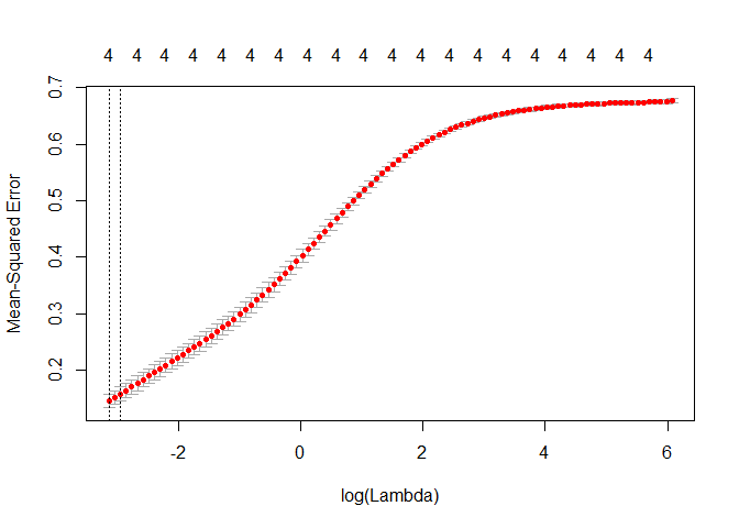
lambda = cv_fit$lambda.min
lambda
## [1] 0.04349958
predicted=predict(cv_fit, as.matrix(iris[,1:4]), s = "lambda.min", type = "class")
u1=union(predicted, iris$Species)
t1 = table(factor(predicted, u1), factor(iris$Species, u1))
confusionMatrix(t1)
## Confusion Matrix and Statistics
##
##
##              setosa versicolor virginica
##   setosa         50          0         0
##   versicolor      0         47         4
##   virginica       0          3        46
##
## Overall Statistics
##
##                Accuracy : 0.9533
##                  95% CI : (0.9062, 0.981)
##     No Information Rate : 0.3333
##     P-Value [Acc > NIR] : < 2.2e-16
##
##                   Kappa : 0.93
##
##  Mcnemar's Test P-Value : NA
##
## Statistics by Class:
##
##                      Class: setosa Class: versicolor Class: virginica
## Sensitivity                 1.0000            0.9400           0.9200
## Specificity                 1.0000            0.9600           0.9700
## Pos Pred Value              1.0000            0.9216           0.9388
## Neg Pred Value              1.0000            0.9697           0.9604
## Prevalence                  0.3333            0.3333           0.3333
## Detection Rate              0.3333            0.3133           0.3067
## Detection Prevalence        0.3333            0.3400           0.3267
## Balanced Accuracy           1.0000            0.9500           0.9450
95%, that’s pretty unrealistic and should be a sign that you did something wrong. I’ll cover that in a second. Let’s see how this compares to an OLS classification model by setting $\lambda = 0$
cv_fit_OLS = glmnet(as.matrix(iris[,1:4]), as.factor(iris$Species),
                           alpha=0, lambda = 0, family = "multinomial")

predicted=predict(cv_fit_OLS, as.matrix(iris[,1:4]), s = "lambda.min", type = "class")
u1=union(predicted, iris$Species)
t1 = table(factor(predicted, u1), factor(iris$Species, u1))
confusionMatrix(t1)
## Confusion Matrix and Statistics
##
##
##              setosa versicolor virginica
##   setosa         50          0         0
##   versicolor      0         49         1
##   virginica       0          1        49
##
## Overall Statistics
##
##                Accuracy : 0.9867
##                  95% CI : (0.9527, 0.9984)
##     No Information Rate : 0.3333
##     P-Value [Acc > NIR] : < 2.2e-16
##
##                   Kappa : 0.98
##
##  Mcnemar's Test P-Value : NA
##
## Statistics by Class:
##
##                      Class: setosa Class: versicolor Class: virginica
## Sensitivity                 1.0000            0.9800           0.9800
## Specificity                 1.0000            0.9900           0.9900
## Pos Pred Value              1.0000            0.9800           0.9800
## Neg Pred Value              1.0000            0.9900           0.9900
## Prevalence                  0.3333            0.3333           0.3333
## Detection Rate              0.3333            0.3267           0.3267
## Detection Prevalence        0.3333            0.3333           0.3333
## Balanced Accuracy           1.0000            0.9850           0.9850
99% is also just as unrealistic as 95%. Why did the ridge perform worse than the OLS model? The OLS is probably over-fitting more than the ridge and that’s due to not splitting the data into a training and testing sets. This is bad practice and I’m doing it here to showcase what happens when you don’t do that.