Props
This document will draw from sources because recreating the wheel isn’t what I’m about. The sources will be listed below:
Danielle Navarro (d.nvarro@unsw.edu.au): https://learningstatisticswithr.com/lsr-0.6.pdf
I’m making a series of posts summarizing basics in statistics for myself and other people who are looking for a quick refresher. I’m filtering out a lot of things that I don’t think practically matter to how we do science. Not to say it doesn’t matter, more to say it doesn’t affect my day to day.
Intro
Why do we need statistics? We need to make objective conclusions about the world. The human brain is ripe with biases that can lead to incorrect conclusions. Statistics helps us come to a consensus about what the “true” answer to a question is.
In 1973, the University of California, Berkeley worried about the admissions of students into their graduate courses. A 9% difference between males and females is definitely a risk in getting sued. At a surface level, it looks like systematic discrimination is occurring.
| Number of applicants | Percent admitted | |
|---|---|---|
| Males | 8442 | 44% |
| Females | 4321 | 35% |
Table: Admission figures for the six largest departments by gender
Department Male Applicants Male Percent Admitted Female Applicants Female Percent admitted
 A               825                   62%                    108                     82%
 B               560                   63%                    25                      68%
 C               325                   37%                    593                     34%
 D               417                   33%                    375                     35%
 E               191                   28%                    393                     24%
 F               373                   6%                     341                     7%
When we actually break it down by department, we can see there are more competitive departments than others. Also, more females apply to the competitive departments than males. Females also have higher acceptance rates and it even looks like there’s a slight bias towards males. This legally clears the university but it doesn’t answer the interesting question of why females are applying to the more competitive courses.
This effect is known as the Simpson’s paradox, not from the show
Mean
You’ve definitely seen this before… The mean is simply every observation summed, divided by the number of observations. This can be mathematically represented like this:
$$\frac 1N\sum_{i=1}^N X_i$$
In R:
data(iris) # load Ronald Fisher Iris dataset
mean(iris$Sepal.Length) #take mean of sepal length
## [1] 5.843333
Median
It’s the middle number. If there isn’t a middle number you take the mean of the adjacent “middle numbers”.
In R:
median(iris$Sepal.Length)
## [1] 5.8
Median v. Mean
Mean is sensitive to outliers in your data so, while the median is not. Taking the median doesn’t actually take in any information about the numbers it just finds the middle one. While the mean actually uses information held in the dataset. If your median is very different from your mean, this could be an indication that there are outliers in your dataset. You should then graph your data to check and then apply the appropriate filters. In the iris dataset, mean and median are comparable so they’re probably aren’t any outliers.
Variability
There are several metrics for this, like range (biggest number - smallest number), interquartile range (75th percentile - 25th percentile). They can be useful and to be honest, I don’t use them. I’m going to skip some of the build up.
In R:
range(iris$Sepal.Length)
## [1] 4.3 7.9
quantile(iris$Sepal.Length)
##   0%  25%  50%  75% 100%
##  4.3  5.1  5.8  6.4  7.9
The range here is 1.5. What R is doing, is adding and subtracting the range from the median and that’s why you see two numbers. It’s the ranges from the median.
Variance
Variance is simply the sum of squares $\sum_{i=1}^N (X_{i} - \overline{X})^2$ divided by the number of observations $\frac{1}{N}$. What’s all the rave about variance? It has some nifty statistical properties that prove useful. One of them is that if you have two sets of data and you calculate the variance of variable A as Var(A) = 125.67 and Var(B) = 340.33 and we want to create variable C which = A + B, the variance of C would 466. This means variances are additive.
We can write the whole equation of variance as:
$$Var(X) = \frac{1}{N-1}\sum_{i=1}^N (X_{i} - \overline{X})^2$$
Where did that -1 come from? It’s a penalization we apply to our estimation of the population variance. Since it’s nearly impossible to ever known the true population variance of the variable, we penalize our estimation of it from the sample that we use.
Variance is all fine and dandy but what does it mean anyway? We can interpret it - obviously large variances can be bad but not always. It does have very good uses for other metrics we’re about to cover.
In R:
var(iris$Sepal.Length)
## [1] 0.6856935
Standard Deviation
Standard deviation is basically an interpenetrate version of variance.
$$\hat{\sigma} = \sqrt{\frac{1}{N-1}\sum_{i=1}^N (X_{i} - \overline{X})^2}$$
It’s simply the square root of the variance equation.
In R:
sd(iris$Sepal.Length)
## [1] 0.8280661
Which is the same as:
sqrt(var(iris$Sepal.Length))
## [1] 0.8280661
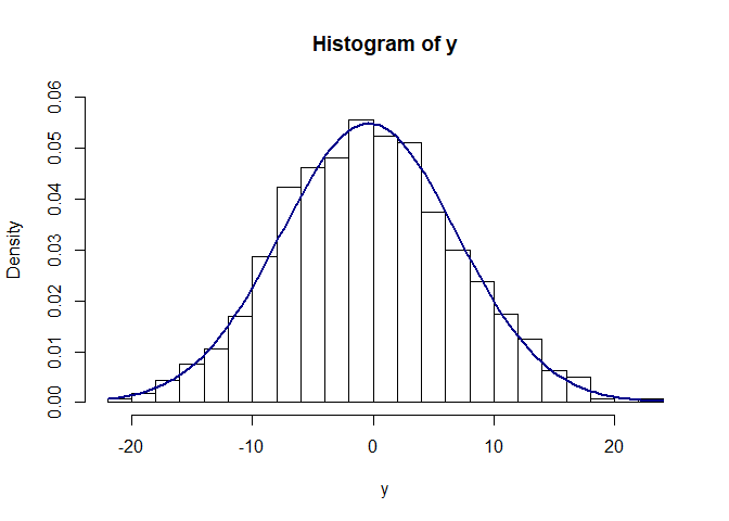
Now I’m assuming if you’ve done a little bit of research and you have a mild understanding and ability to interpret standard deviation. Our interpretation relies on our assumption that our data is normally distributed (I’ll come back to this). This allows us to say within one standard deviation in each direction 67% of will lay in this region.
We would assume our distribution to look something like this:
xseq<-seq(-4,4,.01)
y<-2*xseq + rnorm(length(xseq),0,5.5)
hist(y, prob=TRUE, ylim=c(0,.06), breaks=20)
curve(dnorm(x, mean(y), sd(y)), add=TRUE, col="darkblue", lwd=2)
In the next post, I’ll discuss normality, measures of normality, and sampling.