You might be wondering what’s the best way to determine the number of principal components (PCs) to keep. Is there a more objective method than a scree plot? There are a couple of methods I’ve come across that have stronger quantitative criteria. The one I’ve grown fond of is the broken-stick model, first proposed by MacArthur studying bird species apportionment in different regions. It was then adopted by Frontier to determine how many PCs to keep. Essentially, the species apportionment was translated into variance apportionment compared to PCs.
“The broken-stick model retains components that explain more variance than would be expected by randomly dividing the variance into p parts. If you randomly divide a quantity into parts, the expected proportion of the $k_{th}$ largest piece is (1/p)Σ(1/i) where the summation is over the values i=k..p. For example, if p=7 then
E1 = (1 + 1⁄2 + 1⁄3 + 1⁄4 + 1⁄5 + 1⁄6 + 1⁄7) / 7 = 0.37,
E2 = (1⁄2 + 1⁄3 + 1⁄4 + 1⁄5 + 1⁄6 + 1⁄7) / 7 = 0.228,
E3 = (1⁄3 + 1⁄4 + 1⁄5 + 1⁄6 + 1⁄7) / 7 = 0.156, and so forth.”
This example is from a SAS blog.
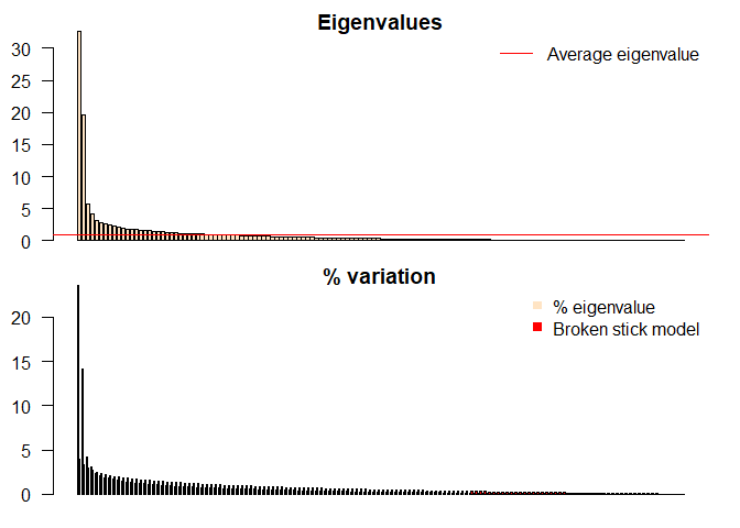
The short and skinny of how to use the broken-stick model is any of the tan bars that are higher than the red bars are the PCs that are kept. Simple enough. In the picture below, the model suggests to keep 4 PCs.
The broken-stick model seems to be one of the go to for selecting the number of PCs. A thing to note is that it does fall on the conservative side of PC selection.
I’ll give a brief description of how to use the broken-stick model below. The code for this can be found on my GitHub.
This function is what will create the barplots comparing eigen values with the broken-stick distribution.
evplot = function(ev) {
# Broken stick model (MacArthur 1957)
n = length(ev)
bsm = data.frame(j=seq(1:n), p=0)
bsm$p[1] = 1/n
for (i in 2:n) bsm$p[i] = bsm$p[i-1] + (1/(n + 1 - i))
bsm$p = 100*bsm$p/n
# Plot eigenvalues and % of variation for each axis
op = par(mfrow=c(2,1),omi=c(0.1,0.3,0.1,0.1), mar=c(1, 1, 1, 1))
barplot(ev, main="Eigenvalues", col="bisque", las=2)
abline(h=mean(ev), col="red")
legend("topright", "Average eigenvalue", lwd=1, col=2, bty="n")
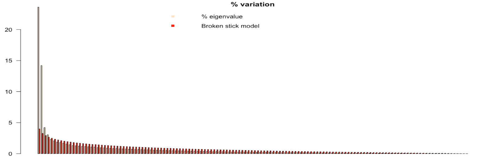
barplot(t(cbind(100*ev/sum(ev), bsm$p[n:1])), beside=TRUE,
main="% variation", col=c("bisque",2), las=2)
legend("topright", c("% eigenvalue", "Broken stick model"),
pch=15, col=c("bisque",2), bty="n")
par(op)
}
Let’s read in our csv file.
HCP = read.csv(file="C:/Users/Mohan/Box/Education_Youtube/Code/Machine Learning/HCP_morph_tutorial_dat.csv", header = TRUE)
And make sure there are no NAs in our dataframe.
HCP = na.omit(HCP)
Run the PCA.
HCP_pca = prcomp(HCP[,4:length(HCP)], center = T, scale. = T)
And create the broken stick model! It will look like the picture below if done correctly.
 ev_HCP = HCP_pca$sdev^2
 evplot(ev_HCP)