One-Way ANOVA
t-tests are fine and dandy but what if you have more than one group? Analysis of variance (ANOVA) will be your hero in this case. Let’s say we have three groups, one who eats veggies, one who eats fruits, and one who eats ramen. We’re interested in level of health. Let’s assume G stands for the # of groups, in this case 3 (G = 3). k will denote a specific group i.e. k = 1, k = 2, k = 3 ($N_k$). N will be the total sample size. Let’s say $N_1 = 5$, $N_2 = 5$, and $N_3 = 5$ so we have N = 15. For simplicity, all of the groups have the same number of observations. This is really only important for more Y will refer to the outcome level or in our case, health level.
ANOVAs are built on the same principles as t-tests. First we must be familiar with variance, which in this case looks like this for multiple groups: $$Var(Y) = \frac{1}{N}\sum_{k=1}^G\sum_{i=1}^{N_k}(Y_{ik}-\overline{Y})^2$$ which can be simplified to $$Var(Y) = \frac{1}{N}\sum_{p=1}^{N}(Y_{p}-\overline{Y})^2$$ where p stands for the observation.
Next we need to have a grasp on sum of squares. ANOVA uses total sum of squares ($SS_{tot}$) which looks like:
$$SS_{tot} = \sum_{k=1}^G\sum_{i=1}^{N_k}(Y_{ik}-\overline{Y})^2$$
So exactly the same as variance but no dividing by the number of observations. $SS_{tot}$ can split up into two kinds of variation: within-group sum of squares ($SS_w$) and between-group sum of squares ($SS_b$). $SS_w$ measures how each person differs from their own groups’ mean mathematically represented by: $$SS_{w} = \sum_{k=1}^G\sum_{i=1}^{N_k}(Y_{ik}-\overline{Y_k})^2$$ $SS_b$ measures the differences between groups mathematically represented by: $$SS_{b} = \sum_{k=1}^GN_k(Y_{k}-\overline{Y})^2$$
Once both of these are computed, we can calculate $SS_{tot} = SS_w + SS_b$. So we’ve captured the variation between groups and within the groups themselves. Now what? We want to compare these sums of squares to each other. First, we’ll have to calculate the degrees of freedoms for groups and observations. $df_b = G - 1$ out case it would equal 2. $df_w = N - G$ and in our case would equal 12. Second we want to compute the mean squares (there are two) by dividing by the degrees of freedom: $$MS_b = \frac{SS_b}{df_b}$$ and $$MS_w = \frac{SS_w}{df_w}$$
Thirdly, we can calculate the F statistic, which is the ANOVA equivalent of the t statistic. We do this by dividing the mean squares between groups by the mean squares within groups: $$F = \frac {MS_b}{MS_w}$$ Similar to the t-test, we find where the F statistic falls on the F distribution based on the degrees of freedom.
Assumptions (they might look familiar):
All groups are normally distributed.
All groups were independently sampled. This means there isn’t one observation in both groups. Or more practically, there are no siblings in your dataset.
The standard deviation between the all groups is the same. In practice, this is almost never true for your data.
Let’s try this in R:
data(iris)
aov_results <- aov(Sepal.Length ~ Species, data=iris)

#easy reporting
#devtools::install_github("easystats/easystats") #this installation takes some time
library(report)
report(aov_results)
## The ANOVA suggests that:
##
##   - The effect of Species is significant (F(2, 147) = 119.26, p < .001) and can be considered as large (partial omega squared = ).
#output table
aov_results %>%
  report() %>%
  to_table()
##   Parameter Sum_Squares DoF Mean_Square        F            p
## 1   Species    63.21213   2  31.6060667 119.2645 1.669669e-31
## 2 Residuals    38.95620 147   0.2650082       NA           NA
##   Omega_Sq_partial
## 1        0.6119308
## 2               NA
I’m a big fan of the easystats initiative. Basically they are creating easy to use tools to report and do statistics, correctly, or at least more correctly. If you’re interested in learning more about easy stats, click on the link!.
Post-hoc testing
ANOVA only detects if there are ANY differences between the groups. We don’t know which differences exist between the groups. Thus, we must do post-hoc testing. Essentially this just doing t-tests. There are several ways to do post-hoc testing. I’ll discuss two methods to do post-hoc testing.
Tukey’s Honest Significant Difference (Tukey-HSD)
Tukey-HSD is a common post-hoc test that controls for type I errors across multiple comparisons. The equation looks like:
$$HSD = q*\sqrt{\frac{MS_w}{n}}$$ Let’s break it down. Find the MS_w, and the number of observations/group. For example if you have 150 observations, 50/group, n = 50. q is found in the q-table. This will give you the HSD. Then you subtract the means of each group from each other and any mean difference larger than the HSD value is significantly different.
In R:
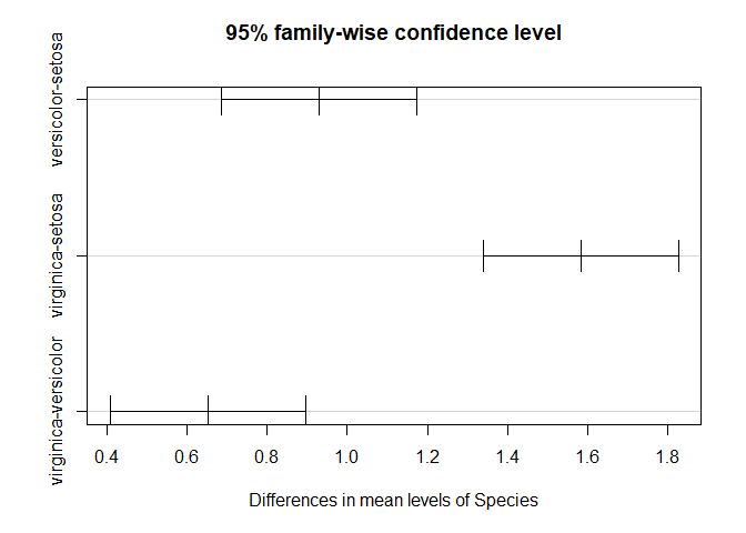
TukeyHSD(aov_results)
##   Tukey multiple comparisons of means
##     95% family-wise confidence level
##
## Fit: aov(formula = Sepal.Length ~ Species, data = iris)
##
## $Species
##                       diff       lwr       upr p adj
## versicolor-setosa    0.930 0.6862273 1.1737727     0
## virginica-setosa     1.582 1.3382273 1.8257727     0
## virginica-versicolor 0.652 0.4082273 0.8957727     0
plot(TukeyHSD(aov_results))
Fisher’s Least Significant Difference (LSD)
LSD is more liberal than Tukey’s test and doesn’t correct for multiple comparisons.
$$LSD_{i-j} = \frac{\hat{\mu_i} - \hat{\mu_j}}{SE}$$ Let’s break this down - i is one group and j is another group. Subtract the mean of one group from the other and divide it by the standard error. The LSD value then works like a t-statistic.
In R:
#install.packages("agricolae")
library(agricolae)
##
## Attaching package: 'agricolae'
## The following object is masked from 'package:report':
##
##     correlation
LSD.test(aov_results, "Species", console=TRUE)
##
## Study: aov_results ~ "Species"
##
## LSD t Test for Sepal.Length
##
## Mean Square Error:  0.2650082
##
## Species,  means and individual ( 95 %) CI
##
##            Sepal.Length       std  r      LCL      UCL Min Max
## setosa            5.006 0.3524897 50 4.862126 5.149874 4.3 5.8
## versicolor        5.936 0.5161711 50 5.792126 6.079874 4.9 7.0
## virginica         6.588 0.6358796 50 6.444126 6.731874 4.9 7.9
##
## Alpha: 0.05 ; DF Error: 147
## Critical Value of t: 1.976233
##
## least Significant Difference: 0.2034688
##
## Treatments with the same letter are not significantly different.
##
##            Sepal.Length groups
## virginica         6.588      a
## versicolor        5.936      b
## setosa            5.006      c
plot(LSD.test(aov_results, "Species"))
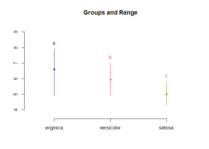
For the function, we have to input the ANOVA model and the groups we’re comparing e.g. “Species”. Groups with the same letter are not significant. In this case, all comparisons are significant.
Multiple Testing Corrections
The LSD post-hoc test doesn’t make any corrections for the number of means compared. Remember the p-value is the probability a difference will be found by chance. If we have an alpha of .05, and we do 3 comparisons, there’s a 15% chance of due to randomness of finding a significant result.
Bonferroni Correction
Let’s say we run 3 post-hoc tests. We would take the p-value of whichever test and multiply it by the number of tests we did, 3, to get the new p value. So if we had $p = 0.01$, it would become $p = 0.05$. Simple enough. $${\alpha\prime} = \frac{\alpha}{k}$$
Where $alpha$ is the chosen significance level, and is the probability of making a type I error. k is the number of tests you’re doing.
In R:
LSD.test(aov_results, "Species", p.adj = "bonferroni", console = T)
##
## Study: aov_results ~ "Species"
##
## LSD t Test for Sepal.Length
## P value adjustment method: bonferroni
##
## Mean Square Error:  0.2650082
##
## Species,  means and individual ( 95 %) CI
##
##            Sepal.Length       std  r      LCL      UCL Min Max
## setosa            5.006 0.3524897 50 4.862126 5.149874 4.3 5.8
## versicolor        5.936 0.5161711 50 5.792126 6.079874 4.9 7.0
## virginica         6.588 0.6358796 50 6.444126 6.731874 4.9 7.9
##
## Alpha: 0.05 ; DF Error: 147
## Critical Value of t: 2.421686
##
## Minimum Significant Difference: 0.2493317
##
## Treatments with the same letter are not significantly different.
##
##            Sepal.Length groups
## virginica         6.588      a
## versicolor        5.936      b
## setosa            5.006      c
plot(LSD.test(aov_results, "Species", p.adj = "bonferroni"))

With bonferroni correction the results are still significant. Note that bonferroni correction is viewed as a very conservative correction and over corrects, increasing your chance of type II errors.
False Discovery Rate (FDR)
FDR changes the p-value to mean only $\alpha$ (5%) discoveries are false rather than each discovery has an $\alpha$ (5%) chance of being false. This looks like: $$FDR = E(V/R | R > 0) P(R > 0)$$ Let’s break it down - Calculate the p-values for each hypothesis test and order from smallest to largest. Then each p-value is multiplied by N and divided by its assigned rank which gives the adjusted p-values. $\alpha$ remains at 0.05.
LSD.test(aov_results, "Species", p.adj = "fdr", console = T)
##
## Study: aov_results ~ "Species"
##
## LSD t Test for Sepal.Length
## P value adjustment method: fdr
##
## Mean Square Error:  0.2650082
##
## Species,  means and individual ( 95 %) CI
##
##            Sepal.Length       std  r      LCL      UCL Min Max
## setosa            5.006 0.3524897 50 4.862126 5.149874 4.3 5.8
## versicolor        5.936 0.5161711 50 5.792126 6.079874 4.9 7.0
## virginica         6.588 0.6358796 50 6.444126 6.731874 4.9 7.9
##
## Alpha: 0.05 ; DF Error: 147
## Critical Value of t: 1.976233
##
## Minimum Significant Difference: 0.2034688
##
## Treatments with the same letter are not significantly different.
##
##            Sepal.Length groups
## virginica         6.588      a
## versicolor        5.936      b
## setosa            5.006      c
plot(LSD.test(aov_results, "Species", p.adj = "fdr"))

As expected with FDR correction, all comparisons are significant.
In the next post, I’ll discuss Linear Regressions.